Paper Explainer: Via Machinae

This is an explainer for my most recent paper, with my Rutgers colleague David Shih, Lina Necib at Caltech, and UCSC grad student (and a Rutgers undergrad alum) John Tamanas. It’s a project that we’ve been working on for a while (some of this being for obvious, 2020-related reasons), and I’m very happy to finally have it see the light of day, as it’s a really interesting convergence of a number of my interests in dark matter-motivated astrophysics, big data, and machine learning.

There’s a lot of moving parts in what we’re doing, so to summarize up front, we are using unsupervised deep learning techniques to discover stellar streams using the dataset of the Gaia telescope. This is the first of (at least) two papers on this idea. This paper is a step-by-step description of how our algorithm (named Via Machinae) works, while the follow up will have our results for the full-sky data.

Motivation

As someone who is interested in dark matter, I’m interested in learning more about the structure of our Galaxy: how stars are distributed and the paths of stellar orbits. Dark matter is the dominant source of gravity for the Galaxy, and so stars can act as tracers for the dark matter potential. At least, in principle.

Of particular interest are stellar streams. Stellar streams are groups of stars that form a line or arc through the Galaxy, all following a common orbit. These streams were created when a gravitationally bound collection of stars (a dwarf galaxy or globular cluster) was pulled apart by the tidal force of the Milky Way. Since every star in the progenitor was nearly at the same position and velocity, their orbits through the Galaxy are nearly identical, resulting in a “line” of stars. These streams are called “cold,” because the process of disruption results in all the stars having nearly the same velocity — and in physics, a collection of particles that has small relative motion looks a lot like an object that is low-temperature (temperature being a measure of internal motion of atoms, after all).

We can use these orderly paths that the streams take through the Galaxy to learn things about the gravitational field of the Galaxy itself. For example, requiring the stars to be pulled by gravity exactly along the line they seem to form places constraints on the distribution of mass. Or, if there are disruptions in the stream of stars — for example, gaps in the stream — that might be a sign that a compact clump of some invisible material passed through.

So, to maybe measure something about dark matter one day, you might be interested in stellar streams. How do we find those?

To trace motion, one needs to measure motion, which is hard for stars. Space is big, and stars are far away, so it is not easy to see a star move over time. But they do move, and with sufficient precision, that movement can be measured. In particular, the the Gaia telescope is a satellite mission that was designed to measure the “proper” motion (that is, motion across the sky) of the nearest billion or so stars in the Milky Way. It does this by repeatedly measuring the position of stars on the sky; over time, that position drifts due to the stellar motion. The angular resolution required is ridiculously good: the Gaia telescope has the resolution to distinguish individual strands of hair of a person standing in San Francisco. From New York City.

Gaia offers an immense dataset: 1.4 billion stars with these proper motion measurements. Stars that are relatively nearby (for the most part stars which are only a few thousand light years away or so) can also get distance measurements: Gaia measures the position of stars while the satellite itself orbits the Earth. As the Earth orbits the Sun, Gaia gets to see the stars from positions separated by 2 AU. The difference in angle to the star as the Earth changes position over the year — the parallax — gives a distance measure. But not all stars have distance measures, and even fewer stars have measures of radial velocity (the motion towards or away from Earth) from Gaia itself (though one can cross reference with surveys which measure redshift, but this isn’t available for every star.

If you had the full 6-dimensional information about the stars kinematics: its position and velocity in the Galaxy, you could look for stellar streams by trying to link of stars that have similar orbits through the Galaxy. This would still be a hard problem (space is big and there are a lot of stars) but as I said, that full information isn’t always available, so you don’t even get to try to solve that problem.

Some of the most successful existing stream-finding algorithms “fill in” that missing information (distance and radial velocity) by leveraging the fact that stars which are in stellar streams were all born in the same environment. Further, these stars all tend to be pretty old: it usually takes a while for a collection of stars to be born, fall into the Galaxy, and get tidally stripped into a stream. So you’re looking not just for a collection of stars in a common orbit, but a collection of stars in a common orbit that all have similar compositions and ages. Since we understand how stars evolve, if you find a collection of old stars, measure their brightness (their magnitude) and how much red light versus blue they emit (their color), you can guess their distance from the Earth, and their radial velocity. Then you can try to find a collection of such stars on a common orbit. But key to that step is the assumption that all the stars in the stream are these old stars, if your stream isn’t made of those, you can’t find them with these approaches.

Finding Weird Things

A while back, I was talking with my colleague David Shih about this problem. There are a huge number of stars in Gaia, with positions on the sky, proper motions, colors, and magnitudes. Somewhere in this haystack are a bunch of streams of stars. But they are hard to find. David has been thinking over the last few years about how to find rare processes at the LHC, using machine learning. One concern there is that we’ve looked for unusual processes (new physics) that we theorists expected to find, but didn’t come up with anything. But what if there is new physics in the data, and it’s just different than what we expected? Maybe we’re missing something.

Recently, he and a physicist at Berkeley, Ben Nachman, had developed an approach to find anomalies in data, without having to know what the anomaly looks like ahead of time. The algorithm is called ANODE, and the idea is as follows.

You have a bunch of data: a collection of “events” each characterized by a set of parameters. We’ll call these parameters “features,” $\vec{x}$. These features could be particle energies and momenta if we’re at the LHC, or stellar positions, proper motions, magnitudes, and colors if we’re thinking about Gaia data.

We imagine that this data is mostly “normal” data — the background. Somewhere hidden within this data is the the anomaly — the signal, the thing we want to find. If we knew the probability distribution of the background and the probability distribution of the dataset as a whole, then the best way to find events that didn’t fit in — i.e., are anomalous — would be to take the following ratio:

\[ R(x) = \frac{P_{\rm data}(x)}{P_{\rm background}(x)}. \]

Wherever $R$ is large, that’s an anomalous event.

That is, you look for events where the probability of finding the event in the real data is much bigger than the probability of finding the event in your model of the background. Those events are weird, and thus interesting. Easy!

Unfortunately, doing this easy thing is hard. Why? Well, for one thing, finding the probability distribution of “normal” events is hard. Even at the LHC, we can only model the collisions of protons so well. For something like a galaxy, which even our best simulations can only give approximations for, much less imitate the actual Milky Way with its specific history? Deriving $P_{\rm background}$ is impossible from first principles.

The data-driven $P_{\rm data}(x)$ is not much better. The problem is that determining a probability density (the distribution of events with specific values of the features) is really hard when the number of features gets above two or three. For features of low dimension, you just make a histogram; but for 4 or 5 or 6 dimensional feature-space? You’d need a ridiculous number of individual events to have enough granularity to make histograms in that space. The “curse of dimensionality” strikes.

What David and Ben realized though, was that we have all these machine learning tools, and they’re pretty damn nifty. In particular, there are a class of deep-learning networks called density estimators, which can learn an arbitrary probability density from a set of data even in very high dimension. I’m not going to describe the process here, but you can read about them elsewhere.

One thing to remember is that machine learning is not AI, and it’s not magic. It’s a set of mathematical steps which can be done only because we have a ridiculous amount of computation available to us these days. It has limits.

So, if you accept for the moment that there are such things called density estimators, and they can learn a probability given a dataset, then in principle we’ve solved half our problem. We can imagine learning $P_{\rm data}(x)$. But that doesn’t solve the problem of having no idea what $P_{\rm background}(x)$ is.

David and Ben’s idea, the basis of ANODE, was that most of the anomalies you’d be interested in are localized in one or more features. A stellar stream, for example, is cold, so all the stars in it have similar proper motions. So, you could imagine training a neural network on the data in one range of the features (where there is no anomaly), and then interpolating that network into a new range of data (where there is an anomaly). The network, having never seen the anomalous dataset, would predict a density distribution as if that anomaly wasn’t there. That is: you’ve got an estimate of $P_{\rm background}(x)$.

That’s a lot, so let me show you an example. In our paper, we use a single stream to walk through the algorithm we’ve developed. That stream is called GD-1. It’s a well-known, very distinct stream (so keep that in mind, compared to other stellar streams, this is easy to find. We’re not using it because it’s tricky, we’re using it because it straightforward and thus well understood). The features of the Gaia data we’re using are: angular position on the sky (two numbers, $\phi$ and $\lambda$), proper motion (two numbers, $\mu_\phi^\ast$ and $\mu_\lambda$), color (one number, $b-r$), and magnitude (one number, $g$). So every star has six numbers. We tile the sky in circles of radius 10 degrees, and take every star in the Gaia data that is further than 1 kpc (3200 light years) away. We exclude stars near the Galactic disk because there are just too many of them. The resulting patches of stars have a few million stars each.

“Via Machinae: Searching for Stellar Streams using Unsupervised Machine Learning” D. Shih, M.R. Buckley, L. Necib, J. Tamanas

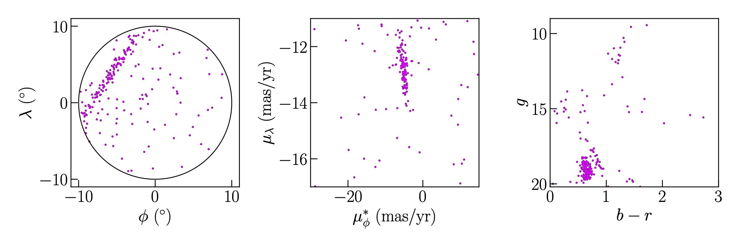
This patch has GD-1 passing through it. You can’t see it, but it’s there. I’ll now overlay the stars which Price-Whelan and Bonaca identified as being likely members of GD-1 (the existence of this catalogue is why we’re using GD-1, as we have something to benchmark against.

Here, I'm coloring the stream stars with red (there are likely some non-stream stars in the bunch, but they're clearly not the dominant group). You can see the stream forms a nice orderly line in position, a strange shape in color-magnitude, and a compact blob in proper motion. That last fact is the "cold" part of a "cold stellar stream."

Here, I'm coloring the stream stars with red (there are likely some non-stream stars in the bunch, but they're clearly not the dominant group). You can see the stream forms a nice orderly line in position, a strange shape in color-magnitude, and a compact blob in proper motion. That last fact is the "cold" part of a "cold stellar stream."

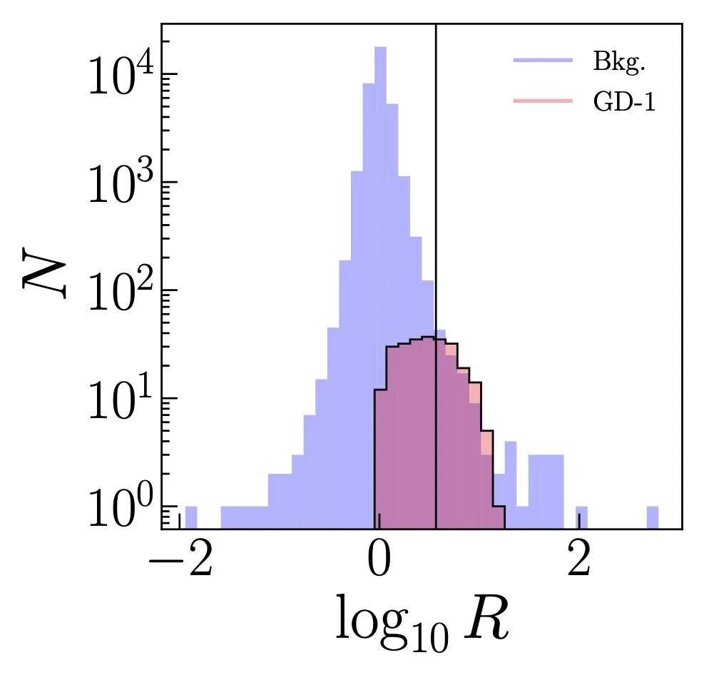
Here's what that looks like. First, here's the distribution of this ratio $R$ for all the stars in the search region shown by the solid black lines in the middle panel above. Red is the distribution of stream star $R$ values, blue is background. If we placed the most optimal cut, requiring very high $R$ values, we'd expect the stream to pop out of the dataset and be visible. First, here's all the stars in the search region (remember, this is a subset of the stars in the above plots). If you know where to look, you can find GD-1, as I said, it is a pretty prominent stream.

Now, here's the same stars, with that cut on $R$. See the stream?

Pretty cool, huh?

Line Finding

We worked this out pretty early on. But then we had a problem. We could apply this density estimation to every range of proper motion in every patch of sky (and we did), and look for anomalies. But I don't know if I mentioned this before, but space is big and there are a lot of stars. Most streams are not as obvious as GD-1, and there are a lot of anomalous collections of stars in the data that aren't streams. We were, frankly, overwhelmed with the number of anomalies we found. We needed a way to narrow down our results to look at things that were likely to be stellar streams. We might be interested in looking for those other weird things some day, but right now we wanted to concentrate on those cold streams made of old stars. We want to find new things, but this kind of new thing.

Our solution to isolate streams in our data is pretty involved. We have to divide the data one the machine learning step is done, and then recombine separate analysis regions in order to cut down on false positives. We had to make a flow-chart. Here it is, but I suggest you read the paper to get all the gory details.

But there's one very cool step I want to draw attention to here. Part of our problem was finding those high-$R$ stars which formed streams in the data. That is: they made lines in the position-space. Finding a line for a human is easy, but how do you automate that?

It turns out there is an old solution to this problem, a machine learning technique that is not deep learning. It's called the Hough transform. If you have a set of points, you can imagine drawing every possible line through every possible point. Those lines will be parametrized by the angle ($\theta$) they make with a set of axes, and their closest approach to the origin ($\rho$). Varying a line through a single point will describe a curve through $\rho-\theta$ space. If there is a set of points in your data that form a line, then their individual curves in this space will all cross at a particular value of $\rho$ and $\theta$: the values that describe the line on which these data points lie.

So, finding a line can be transformed from a problem of drawing a line through a bunch of points (hard) to finding where the most curves in this Hough space cross (easy!). Here's an example (a toy example from a plot that didn't make it into the paper. The GD-1 example is so obvious by eye it kind of obscures how nifty this Hough transform is).

Here, I've dropped a bunch of random fake "stars" in position space, and then a set of stars lying on the same line. Then, I convert all those stars into the Hough space, and draw their curves. I then apply an algorithm that looks for the highest density of curves in some region, which is then identified as the most likely line for the data (and applies a figure-of-merit $\sigma_L$ which estimates how likely this configuration of stars was by random chance. High $\sigma_L$ means it's likely to be a real line.)

This transform and figure of merit allows us to reject anomalous collections of stars that aren't what we're looking for. In our 2nd paper, we're going to show what our results are when we apply this all across the sky, but the first paper, the one that just lays out the step-by-step method of our stream-finding algorithm Via Machinae, we just stick with GD-1.

Refinding GD-1

As I said, we divide the Gaia sky into overlapping patches, within which we look for these cold streams. Our algorithm will stitch together likely stream candidates across patches if they seem to have common features, and if we run this around where we know GD-1 is in the sky, we of course recover this bright stream. Here's the comparison between our algorithm's identification of likely GD-1 stars and the catalogue we benchmarked against (Price-Whelan and Bonaca, 2018).

As you can see, we find most of the stream. On the left side of this plot, we're missing stars, but that was expected. Here, GD-1 gets too close to the disk, and we threw those patches out (the deep learning step takes longer the more stars are in the sample, and there are a lot of stars near the disk). In the middle, we recover many of the known features of GD-1: gaps, high density regions, and an intriguing "spur" that might be the sign of a disruption event in the past (possibly related to dark matter?). One thing to note is our sample of possible stream-stars is a bit less well-defined compared to our benchmark.

This is largely because our algorithm is designed to find streams, but isn't optimized to isolate streams. Once you know where a stream is, you can go back and start pulling the data apart and understanding what you've found. So, when making choices about all the moving parts of Via Machinae, we always erred on the side of making sure we'd find a stellar stream rather than trying to ensure that when we found one, it would have no background stars in it.

You'll also notice we fail to find the right-hand side of the stream. We think we understand why: this region of the stream passed through a single patch of our dataset, and that patch has a lot of stars. The stream stars then were far fewer in proportion to the background in the relevant signal regions. This may be a fundamental limitation of Via Machinae, but we need to look at more example streams to know for sure. But stay tuned: we have the whole sky to cover, and Paper II will be along. Real soon now.