Paper Explainer: ClearPotential: Revealing Local Dark Matter in Three Dimensions

This is a paper explainer for my recent work with my graduate student Eric Putney, previous Rutgers postdoc (now at Institute of Basic Science in Korea), and my Rutgers colleague David Shih. This is the culmination of a series of papers, which I’ve written about here.

The goal of this paper and the larger project is to use the collective motion of the stars near the Earth, as measured by the Gaia Space Telescope, to measure the gravitational potential, acceleration, and mass density of the Milky Way galaxy. In particular, once we have the total mass density, we can subtract off the visible matter (that is, stars and gas, what we call “baryonic” material) to determine the density and distribution of dark matter in the Galaxy.

I’ve explained the behind our work elsewhere, and this paper is the “results” paper that is a partner to this paper. The overall physics idea is that stars in our Galaxy can be thought of a tracers, reacting to the underlying gravitational potential to create a steady-state equilibrium distribution in both position and velocity (the combination of which is called “phase space”). In position-space, that distribution is the familiar bulge-and-disk shape that we think of when we think of spiral galaxies. Gaia is a unique telescope in that it can measure not just where stars are (their angle on the sky, as well as their distance from us), but how they are moving.

If you know the distribution of stars in position and velocity, the phase space density $f(x,v)$, then if we assume the phase space density is in equilibrium, then $f$ obeys the collisionless Boltzmann Equation (CBE): \begin{equation} -v\cdot\nabla f + \nabla\Phi \cdot \frac{\partial f}{\partial v} = 0. \end{equation} Here $\Phi(x)$ is the gravitational potential (which depends only on position), and $\nabla \Phi$ is the derivative of the potential — which is to say the gravitational acceleration.

Estimating the phase space density in position and velocity from data is traditionally a very difficult task; difficult enough that historically we threw our hands up said we couldn’t do it. Instead, we integrated over velocity distributions to get a version of the CBE called the Jeans Equation. But in doing so, you lose information, and even so you have to make a bunch of symmetry assumptions.

The problem is what’s sometimes called the “curse of dimensionality.” If you have a distribution of data in one dimension, you can imagine estimating the density by just making a histogram. Divide the data into bins, count the number of events in the bin, and that’s your phase space estimate. However, there is an error, which is proportional to one over the square root of events in each bin. The more bins (so the more finely you know density), the fewer events in the bin, and the larger the fractional error. But the $f$ the CBE uses has six dimensions (three space, three velocity) no one, and so if you try to histogram the data, each “bin” (a six-dimensional voxel now) has very few datapoints (stars in each bin). That results in large errors, and since the CBE takes derivatives of $f$, the errors in each bin get magnified. This is the curse of dimensionality.

We overcome this problem using machine learning. We use normalizing flows, which are flexible algorithms that learn the most-likely phase space distribution of data in an unsupervised way. The result of the flow is not the true phase space density, but it is a surprisingly good estimate. Much better than any non-deep learning algorithm. Of particular interest, since flows are learned through back-propagation, taking derivatives (as is needed in the CBE) with respect to the input positions and velocities is relatively easy. Once $f$ is known, we can solve for the acceleration at each location from the CBE. The mass density can then be obtained from a derivative of acceleration (a 2nd derivative of the potential): \begin{equation} \nabla^2 \Phi(x) = 4\pi G \rho(x). \end{equation}

We first tried this idea on simulated data, and then on real Gaia data. However, there were limitations to our first approach. First, we didn’t require that our accelerations were actually the derivative of a potential. This meant that our accelerations didn’t have to respect certain physical constraints. For example, they weren’t “curl-free” $\nabla\times a = 0$. The computation was also very slow. We also had a data problem, in that the stars that we measured with Gaia are obscured by dust. This dust artificially reduces our phase space density, meaning what we measure doesn’t respect the CBE.

In our previous paper, we demonstrated a way to solve all these problems. The answer, of course, is more machine learning. We introduce two new neural networks (in addition to the flows which parametrize $f$). One that parametrizes a gravitational potential $\Phi$, and an “efficiency factor” $\epsilon$ that parametrizes the inability to see stars due to dust. As we showed in our previous work, we showed that our efficiency function worked, “erasing” dust from our dataset. In this paper, we show the results for the gravitational potential.

Our data is a set of stars within 4 kpc of the Sun. Further away, Gaia has difficulty measuring the distance to the stars and the velocity of the stars across the sky. So our measurement of the gravity of the Milky Way is restricted to this sphere, which stretches halfway to the Galactic Center (8.1 kpc away), and significantly above and below the stellar disk (which is about 1 kpc thick). But within that sphere, we have a continuous function (parametrized by a neural network) which is capable of evaluating the potential, acceleration, and density at every location. That is, I think, the first time this has been done.

I also want to emphasize that we took into account multiple sources of error, from sources like measurement error, finite statistics, training errors, and correlations in the neural network output. This took a huge amount of time, and Eric spent a lot of time developing new methods to make these error and correlation propagations work.

First up, we can look at the gravitational potential. It looks like this:

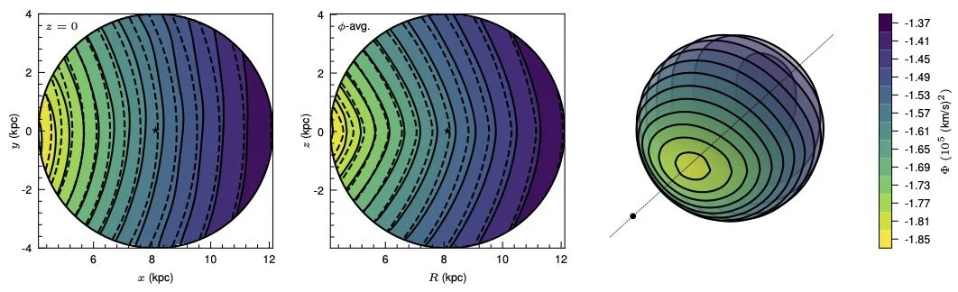
We can compare to a simple model of the Milky Way’s potential, as shown in the plot. We see general agreement, which is expected, and a good sign that our method is working. Deviations from that smooth simple model are either “real” in that the simple model is not capturing the Milky Way potential in a way that we are, or a result of a failure of the data or the assumption of equilibrium. We’ll look at that possibility as we proceed.

Taking a derivative of the potential to get the acceleration. Taking slices through the sphere of data, we see the components of the accelerations here, though remember that we have this a smooth function and could evaluate it anywhere. It’s just hard to visualize.

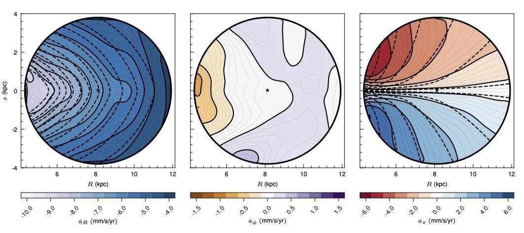
Again, we find decent agreement with the smooth simple model. We again see deviations though. Some of which are incompatible with the assumption of equilibrium. In particular the acceleration component in the direction “around” the disk should be zero in equilibrium. We measure non-zero components, especially towards the Galactic Center (likely due to our dust removal being imperfect). We also see “ledges” in the radial acceleration around the edge of the disk. These may not be dust-related, and could be the result of disequilibrium.

One way to test this disequilibrium is to get a separate measurement of acceleration, one that doesn’t require the equilibrium assumption. Of course, if we had that everywhere, we wouldn’t need to do all the work we just did. But we don’t have it everywhere. What we can compare to are the line-of-sight accelerations for specific pulsars which live in binary systems. There are 24 such systems, measured by Donlon et al and Moran et al.

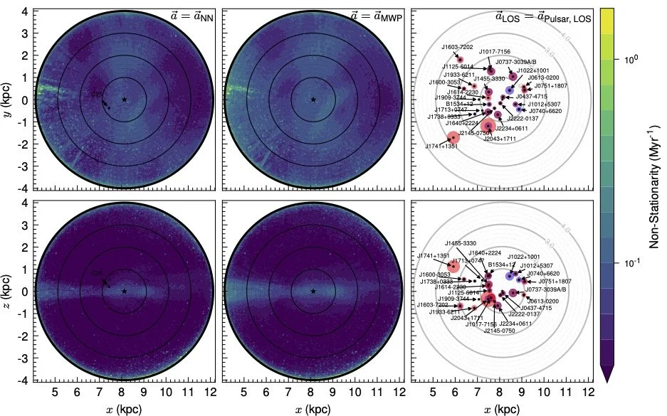
Comparing our accelerations to the pulsar line-of-sight accelerations, we find good but not exact agreement. However, we don’t see any obvious pattern of disagreement which would be suggestive of some unexpected localized gravitational source (that is, something other than the expected dark matter within the Milky Way). We can also use a “non-stationary” metric, which quantifies whether our CBE solution is actually zero. Larger values of this metric say we’re not getting self-consistent answers from the networks. We can do this in two ways, either using “our” accelerations (the result of the network) or the accelerations from the pulsar measurements. In either case, we see suggestions of disequilibrium due to dust towards the Galactic Center. However, there are also signs of larger-than-expected non-stationarity within the disk near us, in regions that are not obviously dust-dominated. This requires more study; some of this is likely that the stars are themselves not in equilibrium due to processes of star formation and evolution within the disk, but some of it may be due to interesting substructure.

Finally, we turn to the mass density. Most interesting to me, we are at a point where the measurement of dark matter in the disk is now dominated by our lack of knowledge of the baryonic mass distribution. If we just evaluate the neural networks at the location of the Sun, we get a terrible measurement of the dark matter density: $\rho_\odot = (-1.71 \pm 1.43)\times 10^{-2} M_\odot/pc^3$. The giant error bar relative to the negative value tell you this result is highly uncertain. A significant part of this error is due to the baryonic error, but not all of it.

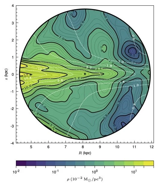
While the measurement at any single location has large uncertainty, if we make assumptions about the symmetry of the dark matter distribution, we can average over multiple locations and get more accurate results. For example, if we average over the plane of the disk (assuming that dark matter density only depends on height above the disk and distance from the center, which is the equilibrium result), we get a map of dark matter like what you see to the right.

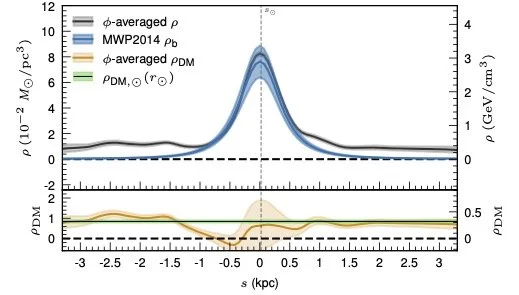
Slicing through the sphere at the Solar radius, we map the total and dark matter densities moving above and below the disk (again assuming azimuthal symmetry). You can see the errors getting large within the disk, but there is clear evidence above and below the disk (where there are few baryons) that the CBE requires a form of mass density that is not accounted by the baryons — that is, dark matter. With this averaging, we find $\rho_\odot = (0.84 \pm 0.08)\times 10^{-2} M_\odot/{\rm pc}^3$, or $0.32\pm 0.03 {\rm GeV/cm^3}$ in particle-physics units. This is a bit smaller than other measurements, but it is where the data takes us.

The thing I want to emphasize here is that we can make very good measurements of the total mass density well away from the Galactic plane. Far from the disk, there are very few baryons: few stars, not much gas, not much dust. Even though our baryonic model is not perfect, we can’t be wrong about the amount of visible matter there by orders of magnitude. And our method very clearly finds significant dynamical evidence for mass density. That’s dark matter.

We can then average over angles to estimate the dark matter density at each radius (from the Galactic Center) within our sphere of data. Again, there are symmetry assumptions here, but it allows us to test models of dark matter density distributions, like the Navarro-Frenk-White (NFW) profile or a more flexible triaxial model. We find in all cases some preference for a relatively short scale radius, though it must be said that we don’t really have enough of a level arm close to the Galactic Center to have a lot of statistical power here.

In all these fits, we had to include the full correlations of the neural network fits to data, as well as the baryonic model. This is something that sounded easy when we were talking about how to do it, but turned in to a very finicky and computationally complex problem. Eric spent a huge amount of time making this problem tractable, but I think the work paid off.

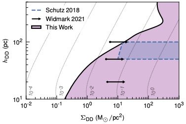
As our very last test, we look for evidence for a “dark disk”: a disk of dark matter that is co-local to the baryonic disk. This shouldn’t happen in “simple” dark matter models, but could in more exotic scenarios. We’re limited by the uncertainty in the baryonic model, but we still set world-leading constraints, especially for very narrow disks — again, this is only possible because of our control over the correlations in our results.

So there you have it: a fully differentiable, continuous model of dark matter within the local volume around the Sun, looking through the dust in the Galaxy. This is completely data driven, using machine learning to solve a physics-inspired neural network (a PINN), whose loss function is just a statistical mechanics equation. In the future, we want to get closer to the Galactic Center, and understand more what the signatures of real disequilibrium in our results would look like. And if anyone has a better model of the baryons, that would really help.